12  TP53 myeloid neoplasms

12.1 Biology of TP53

12.1.1 Nonmutational p53 dysfunction in MDS

• Study Overview: Investigated p53 dysfunction in myelodysplastic syndromes (MDS) through mutational and nonmutational mechanisms.(Zampini et al. 2025)

• Analyzed 6,204 MDS patients (Cohort 1), with subsets for RNA sequencing (n=109), immune cell phenotyping (n=77), and single-cell multiomics (n=15).

• Validated findings in an independent cohort of 914 patients (Cohort 2).

• TP53 Mutations and Prognosis: TP53 mutations found in 10.1% of patients; biallelic inactivation strongly drove disease progression, identifying high-risk patients regardless of variant allele frequency (VAF).

• Monoallelic TP53 inactivation showed intermediate prognosis, worse than wild-type (wt) but better than biallelic (P<.001).

• Biallelic and monoallelic inactivation represent stages of a multihit process, with 18/23 monoallelic patients progressing to biallelic status at AML evolution.

• Nonmutational p53 Dysfunction: Identified 5% of MDS patients with TP53wt but hyperexpression of abnormal p53 protein in bone marrow progenitors, showing poor outcomes similar to biallelic TP53 inactivation.

• Associated with upstream signaling aberrations in PI3K, RAS, WNT, NF-kB pathways, and MDM2 gene amplification (3/10 cases).

• Immunohistochemical p53 hyperexpression (4.1% of 2,500 patients) correlated with dismal prognosis, validated in multivariable analyses.

• Transcriptomic and Immunological Insights: RNA sequencing of CD34+ cells revealed similar transcriptomic profiles in TP53 biallelic and TP53wt with p53 hyperexpression, with downregulated p53 target genes (P<.001).

• Immune dysregulation in p53 dysfunction included myeloid-derived inflammation, impaired antigen presentation, and downregulated MHC class II and IFNγ pathways.

• Single-cell CITE-seq confirmed immune evasion (upregulated PD-L1, CD39) and T-cell exhaustion (increased PD-1, CD39) in MDS with p53 dysfunction.

• Clinical Implications: Nonmutational p53 dysfunction patients should be managed similarly to biallelic TP53 cases, potentially refining therapeutic timing (e.g., earlier HSCT for monoallelic patients).

• Conventional prognostic scores (IPSS-R, IPSS-M) may underestimate risk in monoallelic and nonmutational p53 dysfunction cases.

• Immunohistochemistry for p53/MDM2 proposed as a diagnostic marker for routine work-up.

• Therapeutic and Research Directions: Distinct immunosuppressive profile suggests potential for immunotherapies targeting myeloid-derived inflammation and immune checkpoints.

• Transcriptomic signature (253 genes) accurately identified p53 dysfunction (96% accuracy), validated across Humanitas, TCGA, and BeatAML cohorts.

• Calls for mechanistic classification of MDS using multiomics to improve risk assessment and clinical trial design.

• Study Support and Affiliations: Conducted by GenoMed4All, Synthema, Synthia, and icMDS consortia, supported by EU-Horizon 2020/2023, AIRC, and other grants.

12.2 Treatments

12.2.1 Inqovi (oral decitabine)

ASH 2024 abstract: Propensity score matching (Urrutia et al. 2024)

# Load required libraries
library(tidyverse)

── Attaching core tidyverse packages ──────────────────────── tidyverse 2.0.0 ──
✔ dplyr     1.2.1     ✔ readr     2.2.0
✔ forcats   1.0.1     ✔ stringr   1.6.0
✔ ggplot2   4.0.3     ✔ tibble    3.3.1
✔ lubridate 1.9.5     ✔ tidyr     1.3.2
✔ purrr     1.2.2     
── Conflicts ────────────────────────────────────────── tidyverse_conflicts() ──
✖ dplyr::filter() masks stats::filter()
✖ dplyr::lag()    masks stats::lag()
ℹ Use the conflicted package (<http://conflicted.r-lib.org/>) to force all conflicts to become errors

library(kableExtra)

Attaching package: 'kableExtra'

The following object is masked from 'package:dplyr':

    group_rows

library(gt)

# Create summary data frame based on the study results
mds_summary <- data.frame(
  Group = c("TP53wt", "TP53single-hit", "TP53multi-hit"),
  
  # Patient characteristics
  N = c(107, 50, 23),
  Percent = c(59.5, 27.8, 12.7),
  Complex_Cytogenetics_Pct = c(NA, NA, 69.5),
  Median_Comutations = c(4, 3, 2.5),
  Comutations_IQR = c("3-6", "1-5", "2-3"),
  
  # Response characteristics
  Complete_Response_Rate = c(NA, NA, NA),  # Not specified in abstract
  No_Response_Pct = c(27.1, 28, 39.1),
  
  # Treatment duration
  Median_Courses = c(9, 7.5, 5),
  
  # Time to loss of response
  Time_to_Loss_Response_mo = c(15.1, 13.2, 8.2),
  
  # Survival
  Median_OS_mo = c(31.7, 22.1, 11.5),
  OS_95CI = c("19.5-51.1", "14.6-35.9", "8.6-19.1")
)

# Create a formatted table using gt
summary_table <- mds_summary %>%
  gt() %>%
  tab_header(
    title = "Summary of Oral Decitabine/Cedazuridine in MDS Patients by TP53 Status",
    subtitle = "Data from Phase II and III Trials"
  ) %>%
  tab_spanner(
    label = "Patient Characteristics",
    columns = c(N, Percent, Complex_Cytogenetics_Pct, Median_Comutations, Comutations_IQR)
  ) %>%
  tab_spanner(
    label = "Treatment Response",
    columns = c(Complete_Response_Rate, No_Response_Pct, Median_Courses, Time_to_Loss_Response_mo)
  ) %>%
  tab_spanner(
    label = "Survival Outcomes",
    columns = c(Median_OS_mo, OS_95CI)
  ) %>%
  cols_label(
    N = "N",
    Percent = "%",
    Complex_Cytogenetics_Pct = "Complex Cytogenetics (%)",
    Median_Comutations = "Median Co-mutations",
    Comutations_IQR = "Co-mutations (IQR)",
    Complete_Response_Rate = "CR Rate (%)",
    No_Response_Pct = "No Response (%)",
    Median_Courses = "Median Courses",
    Time_to_Loss_Response_mo = "Time to Loss of Response (mo)",
    Median_OS_mo = "Median OS (mo)",
    OS_95CI = "95% CI"
  ) %>%
  fmt_missing(
    columns = everything(),
    missing_text = "NR"
  ) %>%
  tab_source_note(
    source_note = "NR = Not Reported; OS = Overall Survival; CR = Complete Response"
  ) %>%
  tab_footnote(
    footnote = "p = 0.002 for comparison of median co-mutations across groups",
    locations = cells_column_labels(columns = Median_Comutations)
  ) %>%
  tab_footnote(
    footnote = "p = 0.016 for comparison across groups",
    locations = cells_column_labels(columns = Median_Courses)
  ) %>%
  tab_footnote(
    footnote = "p < 0.005 for log-rank test across groups",
    locations = cells_column_labels(columns = Median_OS_mo)
  )

Warning: Since gt v0.6.0 `fmt_missing()` is deprecated and will soon be removed.
ℹ Use `sub_missing()` instead.
This warning is displayed once every 8 hours.

# Display the table
summary_table

Summary of Oral Decitabine/Cedazuridine in MDS Patients by TP53 Status
Data from Phase II and III Trials
Group	Patient Characteristics					Treatment Response				Survival Outcomes
	N	%	Complex Cytogenetics (%)	Median Co-mutations1	Co-mutations (IQR)	CR Rate (%)	No Response (%)	Median Courses2	Time to Loss of Response (mo)	Median OS (mo)3	95% CI
TP53wt	107	59.5	NR	4.0	3-6	NR	27.1	9.0	15.1	31.7	19.5-51.1
TP53single-hit	50	27.8	NR	3.0	1-5	NR	28.0	7.5	13.2	22.1	14.6-35.9
TP53multi-hit	23	12.7	69.5	2.5	2-3	NR	39.1	5.0	8.2	11.5	8.6-19.1
1 p = 0.002 for comparison of median co-mutations across groups
2 p = 0.016 for comparison across groups
3 p < 0.005 for log-rank test across groups
NR = Not Reported; OS = Overall Survival; CR = Complete Response

# Create propensity score matching results table
psm_results <- data.frame(
  Treatment = c("Decitabine/Cedazuridine", "IV HMA"),
  N = c(47, 47),
  Median_OS_mo = c(13.1, 8.0),
  OS_95CI = c("8.4-21.3", "5.2-13.0"),
  P_value = c("0.047", "Reference")
)

# Create PSM results table
psm_table <- psm_results %>%
  gt() %>%
  tab_header(
    title = "Propensity Score Matched Analysis",
    subtitle = "TP53-mutated MDS Patients"
  ) %>%
  cols_label(
    Treatment = "Treatment",
    N = "N",
    Median_OS_mo = "Median OS (months)",
    OS_95CI = "95% CI",
    P_value = "P-value"
  ) %>%
  tab_footnote(
    footnote = "Matched on age, ECOG PS, IPSS-R scores, and TP53 VAF",
    locations = cells_column_labels(columns = Treatment)
  ) %>%
  tab_footnote(
    footnote = "Log-rank test",
    locations = cells_column_labels(columns = P_value)
  )

# Display PSM table
psm_table

Propensity Score Matched Analysis
TP53-mutated MDS Patients
Treatment1	N	Median OS (months)	95% CI	P-value2
Decitabine/Cedazuridine	47	13.1	8.4-21.3	0.047
IV HMA	47	8.0	5.2-13.0	Reference
1 Matched on age, ECOG PS, IPSS-R scores, and TP53 VAF
2 Log-rank test

# Alternative: Create a simple summary using base R
cat("=== STUDY SUMMARY ===\n")

=== STUDY SUMMARY ===

cat("Total patients analyzed: 180\n")

Total patients analyzed: 180

cat("Patients with TP53 mutations: 73 (40.5%)\n")

Patients with TP53 mutations: 73 (40.5%)

cat("- TP53 wild-type: 107 (59.5%)\n")

- TP53 wild-type: 107 (59.5%)

cat("- TP53 single-hit: 50 (27.8%)\n")

- TP53 single-hit: 50 (27.8%)

cat("- TP53 multi-hit: 23 (12.7%)\n\n")

- TP53 multi-hit: 23 (12.7%)

cat("Median follow-up: 21.5 months\n")

Median follow-up: 21.5 months

cat("HSCT at 4-month landmark: No survival improvement\n\n")

HSCT at 4-month landmark: No survival improvement

# Create a visualization of overall survival
library(ggplot2)

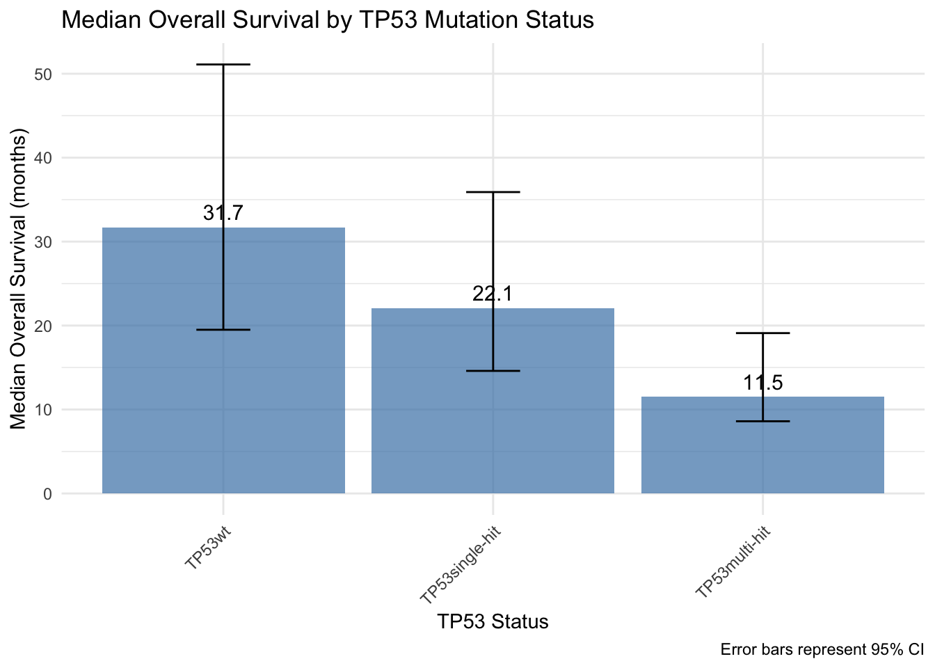
os_data <- data.frame(
  Group = factor(c("TP53wt", "TP53single-hit", "TP53multi-hit"),
                 levels = c("TP53wt", "TP53single-hit", "TP53multi-hit")),
  Median_OS = c(31.7, 22.1, 11.5),
  Lower_CI = c(19.5, 14.6, 8.6),
  Upper_CI = c(51.1, 35.9, 19.1)
)

os_plot <- ggplot(os_data, aes(x = Group, y = Median_OS)) +
  geom_col(fill = "steelblue", alpha = 0.7) +
  geom_errorbar(aes(ymin = Lower_CI, ymax = Upper_CI), 
                width = 0.2, 
                position = position_dodge(0.9)) +
  labs(title = "Median Overall Survival by TP53 Mutation Status",
       x = "TP53 Status",
       y = "Median Overall Survival (months)",
       caption = "Error bars represent 95% CI") +
  theme_minimal() +
  theme(axis.text.x = element_text(angle = 45, hjust = 1)) +
  geom_text(aes(label = round(Median_OS, 1)), 
            vjust = -0.5, 
            size = 4)

# Display the plot
print(os_plot)

12.2.2 Magrolimab

12.2.2.1 ENHANCE-2

12.2.3 STING Agonists

12.2.4 Entrectinib and ASTX727

12.2.5 Immunotherapy in TP53 myeloid neoplasms

12.2.6 Rezatapopt (PC14586)

• a First-in-Class, Small-Molecule Reactivator of p53 Y220C Mutant in Development (Vu et al. 2024)

Urrutia, Samuel, Koji Sasaki, Alex Bataller, et al. 2024. “Oral Decitabine/Cedazuridine in Patients with MDS and TP53 Mutations: A Propensity Score Matching Analysis from the Phase II and III Trials.” Blood 144 (Supplement 1): 661–61. https://doi.org/10.1182/blood-2024-193274.

Vu, Binh T., Romyr Dominique, Bruce J. Fahr, et al. 2024. “Discovery of Rezatapopt (PC14586), a First-in-Class, Small-Molecule Reactivator of P53 Y220C Mutant in Development.” ACS Medicinal Chemistry Letters 16 (1): 34–39. https://doi.org/10.1021/acsmedchemlett.4c00379.

Zampini, Matteo, Elena Riva, Luca Lanino, et al. 2025. “Characterization and Clinical Implications of P53 Dysfunction in Patients with Myelodysplastic Syndromes.” Journal of Clinical Oncology, ahead of print, May 2. https://doi.org/10.1200/jco-24-02394.